A group project for the university course Financial Time Series, in which we systematically built and backtested SPX option strategies over 25 years and combined them into a tail-aware Markowitz portfolio.

---

Harvesting the Volatility Risk Premium

Group members: Tom Köhler, Sebastian Jung and me.

Stack: Python, Rust (via Maturin), Optuna, GJR-GARCH, WRDS OptionMetrics

The Question

The Variance Risk Premium (VRP), meaning the persistent gap between options-implied volatility and realized volatility, is one of the most studied “free lunches” in finance. The catch is that harvesting it naively means selling insurance into every market crash. The strategies look fantastic until they don’t.

For our project we asked two questions:

1. Does the VRP actually survive a careful, tail-aware backtest across six different SPX option structures over 25 years?
2. If we mix these strategies into a Markowitz-optimal portfolio, are the resulting weights stable, or just an artifact of the specific path of crashes in our sample?

The Data

We built a survivorship-bias-free pipeline on top of WRDS OptionMetrics, spanning the years 1996 to 2025. This window covers the Dot-Com bubble, the 2008 GFC, the 2020 COVID crash, and the post-COVID inflation regime.

Source	Series
WRDS	SPX option chains (calls & puts), daily
Yahoo Finance	SPX, 7 benchmark ETFs (VOO, GLD, VNQ, PDBC, EuroStoxx50, MSCI Asia, US 10Y), risk-free rate (^IRX)
GJR-GARCH(1,1,1)	Out-of-sample 30-day volatility forecast

The raw options data is notoriously noisy and full of stale quotes, untradable spreads, and penny-priced wings. We applied a strict liquidity filter: a ±30% moneyness band, a 100-day DTE cap, and the elimination of contracts with zero volume, zero open interest, or missing greeks. The backtest officially starts on January 19, 1999, the first trading day after the third Friday of January, so that every strategy enters the market on a fresh monthly expiration cycle.

The Strategies

We tested six option structures, ranging from defensive premium-collection plays to a custom volatility-timing model:

• Covered Call: long stock plus short OTM call. Income with capped upside.
• Short Put (1-DTE): sells short-dated puts to harvest theta. High win-rate, brutal tails.
• Short Strangle: sells OTM call and put. Pure short-volatility.
• Long Strangle: the inverse, with long convexity and slow theta bleed.
• Calendar Spread: sells near-term, buys longer-dated at the same strike. Long vega.
• VRP Strangle (our custom strategy): a dynamic short strangle that only fires when our econometric VRP signal flags options as overpriced.

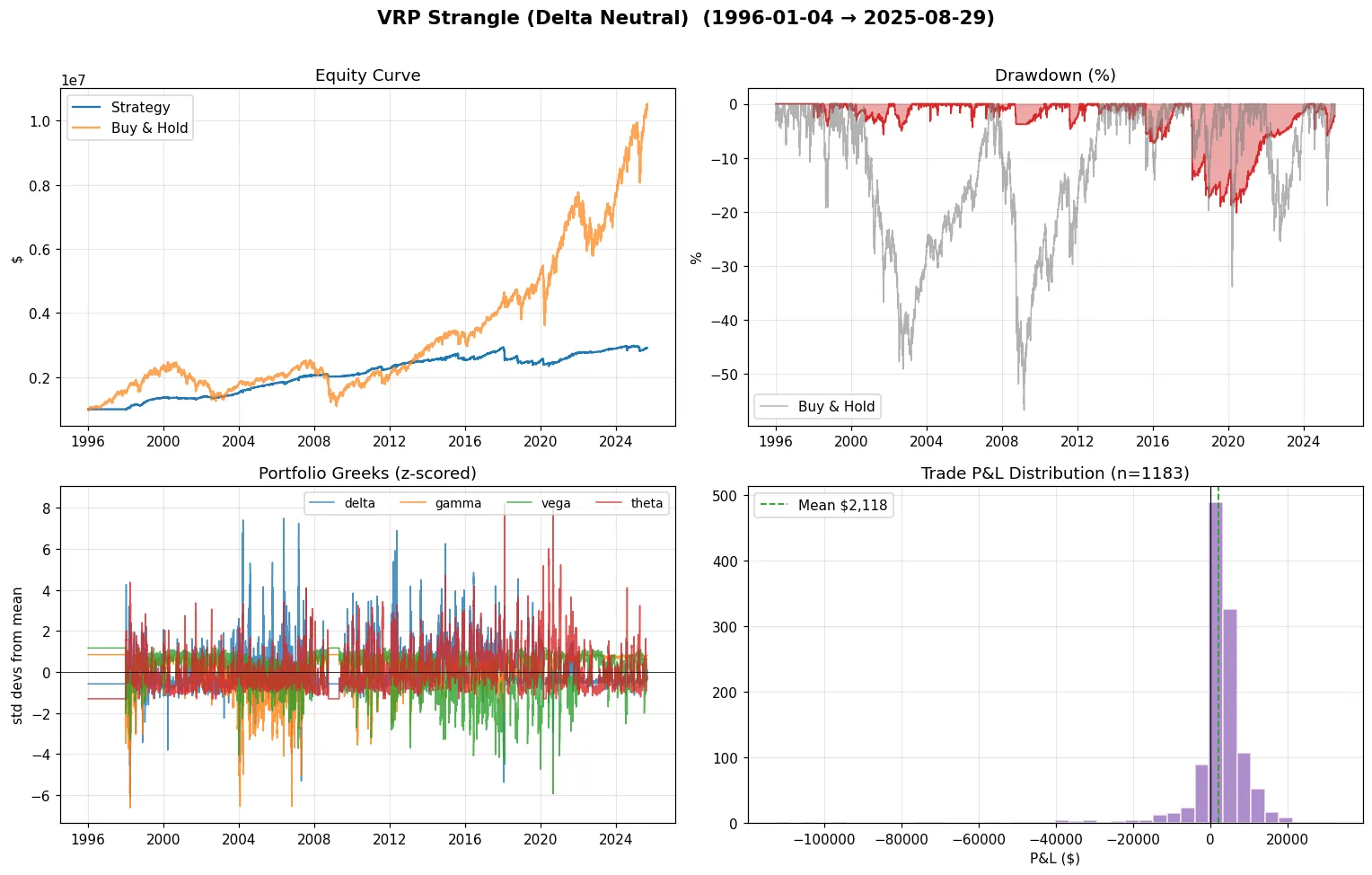
The VRP Strangle

The VRP Strangle is the centerpiece of the project. It runs an asymmetric GJR-GARCH(1,1,1) model on a rolling 504-day window of SPX returns to forecast 30-day volatility, then compares that forecast to the market-implied ATM IV:

$\text{VRP Ratio}_t = \frac{\text{IV}_t^{\text{ATM}}}{\hat{\sigma}_{t,30}^{\text{GARCH}}}$

When the ratio breaches a tuned threshold, the strategy opens a short strangle. Strikes are placed dynamically, at a multiple of the GARCH-forecasted standard deviation rather than a fixed delta, so the wings widen automatically when the model expects more turbulence.

Crucially, the strategy is delta-hedged conditionally. Hedging only kicks in when annualized GARCH volatility exceeds 20%, and only when the absolute portfolio delta drifts beyond a tolerance band. This avoids the round-trip transaction costs of constant rebalancing while still cutting tail exposure during stress regimes.

Engineering: Rust Made This Possible

Options backtesting is path-dependent. You have to step chronologically through the data to manage open positions, which means heavy stateful Python loops. Hooking that up to Optuna for hyperparameter tuning produced runtimes in the multi-hour range per strategy.

We rewrote the inner loop in Rust and exposed it to Python via Maturin:

• Zero-copy NumPy access, so no marshaling overhead between languages.
• Pre-grouped option chains by trading day, so no full-dataset scans per query.
• GIL release for true multi-threading, so Optuna trials parallelize across all cores.

End result: a greater than 40x speedup. Hours became minutes. We could explore far more of the search space without losing the day to a progress bar.

Optimization: Optuna and Walk-Forward

For five of the strategies, we used Optuna’s TPE sampler over the full 25-year sample to optimize entry DTE, target delta, and exit timing. For the VRP Strangle, full-sample optimization is too dangerous because the model is reactive enough that it will overfit to the specific sequence of crashes. We therefore ran a stricter 4-Fold Walk-Forward scheme (60% train, 40% validation) with a final 30% held-out blind set.

Headline base-backtest results (un-optimized parameters):

Strategy	CAGR	Sharpe	Max DD
SPX Buy & Hold	+8.24%	0.51	−56.78%
Covered Call	+1.31%	0.45	−9.20%
Short Put 1-DTE	+0.36%	0.37	−3.77%
Short Strangle	+0.61%	0.39	−6.48%
Long Strangle	−1.14%	−0.52	−28.82%
Calendar Spread	+0.34%	0.12	−12.52%
VRP Strangle	+3.68%	0.98	−20.20%

Two things stand out. First, the Long Strangle is the only strategy with a negative CAGR, which is itself a clean validation of the VRP. Buying gamma persistently loses to theta decay. Second, the VRP Strangle’s drawdown is less than half the SPX’s, with a higher Sharpe than every other strategy and the benchmark. The Long Strangle was dropped from the portfolio.

Portfolio Construction: Why CVaR, Not Variance

Mean-variance optimization has a closed-form solution but penalizes upside and downside symmetrically, which is a terrible fit for option-selling P&L where the left tail is everything. We replaced variance with CVaR-99, the average loss on the worst 1% of trading days. CVaR is a coherent risk measure and directly targets the kind of risk that actually matters here.

Rather than solving analytically, we sampled. We drew 100,000 long-only weight vectors from a Dirichlet(1,…,1), which is uniform over the simplex, and capped each weight at 20% to force diversification. Without the cap, the optimizer concentrates almost everything in whichever asset got luckiest in-sample, usually Gold.

For each sampled portfolio we computed CAGR and CVaR-99, then plotted the cloud:

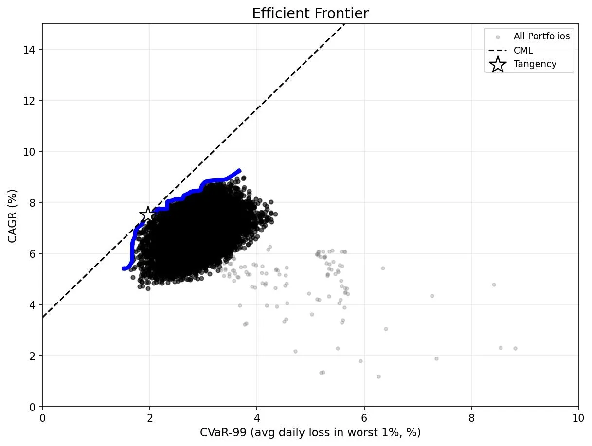
The red star is the tangency portfolio, the one that maximizes the CVaR-Sharpe ratio at a forward-looking $r_f = 3.5\%$ (roughly the current 1-month T-bill yield).

Results

The tangency portfolio’s equity curve, compared to an SPX buy-and-hold:

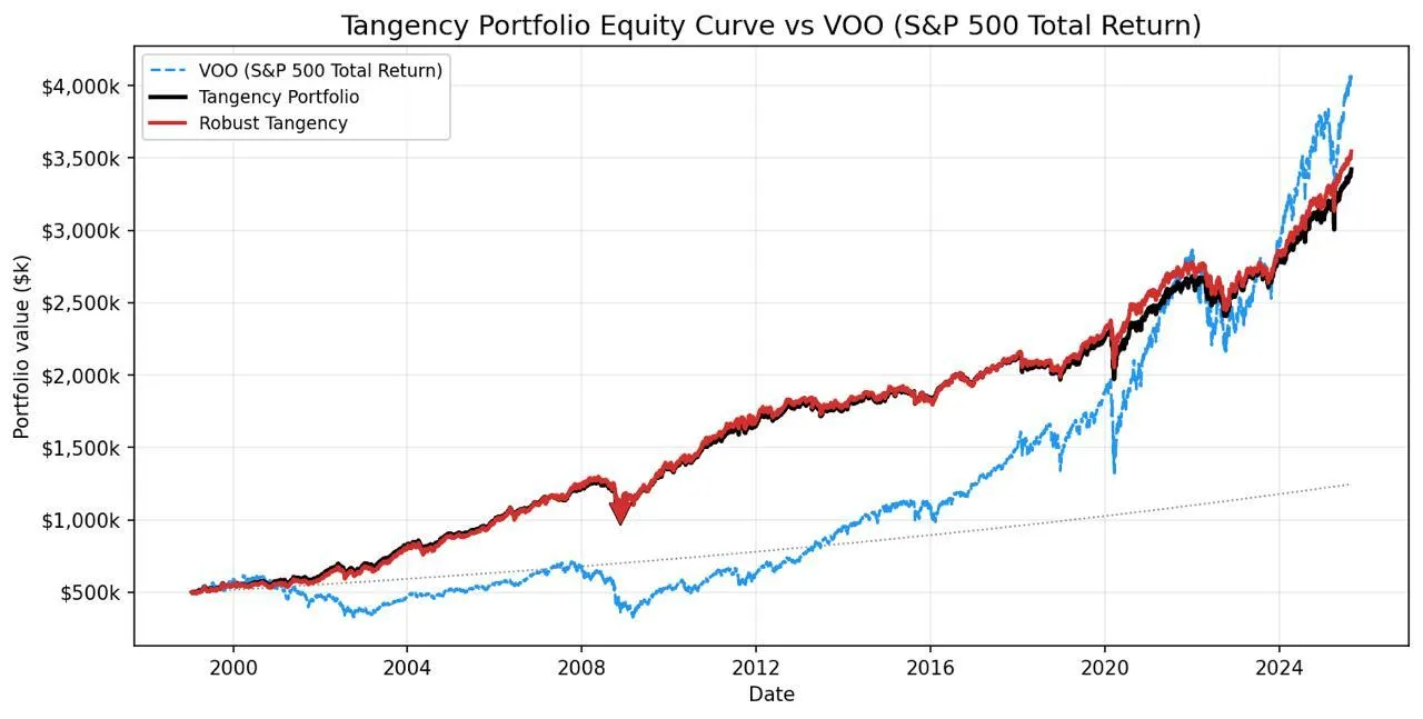
Portfolio	CAGR	CVaR-99	CVaR-Sharpe
Tangency	+7.5%	1.96%	2.04x
Robust Tangency	+7.5%	1.87%	2.15x
SPX Buy & Hold	+8.24%	n/a	n/a (Max DD: −56.78%)

We give up roughly 70 bps of CAGR versus SPX in exchange for an approximately 28x reduction in worst-case loss. That is the bargain on offer here, and it is a good one.

Robustness: Are These Weights Real?

Any 25-year sample contains only about four major tail events. With so few crashes, the optimizer can easily memorize them. To test whether the tangency weights are a fundamental property of the assets or just an artifact of this specific path, we block-bootstrapped monthly returns (60 resamples) and re-ran the optimization on each.

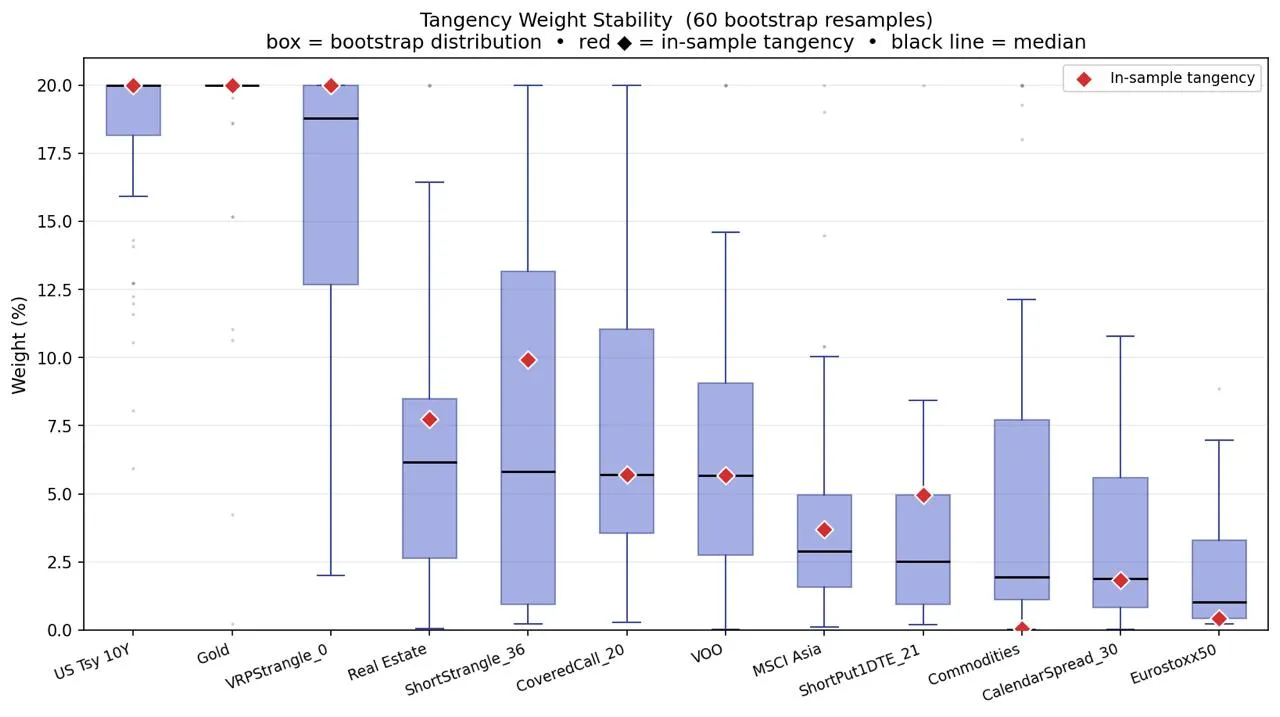
The robustified weights tell a clean story:

• The two highest-tail-risk strategies got trimmed: ShortStrangle (down 3.6pp) and ShortPut1DTE (down 2.2pp). The optimizer was overweighting them in-sample.
• Defensive diversifiers were strengthened: Commodities entered from 0% (+2.0pp), Treasuries and Gold both ticked up (+1.6pp).
• The core anchors held: VRPStrangle, US 10Y Treasuries, and Gold all sit at the 20% cap across nearly every resample. These are stable allocations, not lucky ones.

The robust tangency portfolio matches the in-sample CAGR (+7.5%) but with lower CVaR (1.87% versus 1.96%). Resampling didn’t cost us return; it improved tail efficiency.

Takeaways

The VRP is real, persistent, and harvestable, but only if you respect the tails. A naive short-volatility book is a leveraged bet that the next crash never comes. Three design choices made the difference here:

1. Conditional entry via GJR-GARCH. Only sell vol when the econometric model says it’s actually overpriced, not on a fixed schedule.
2. CVaR-based portfolio construction. Explicitly penalize left-tail exposure, which variance does not.
3. Bootstrapping the weights. Let the optimizer’s overconfidence in lucky in-sample tail behavior get washed out by resampling.

The final portfolio gives up a small amount of expected return for a dramatic reduction in drawdown risk, and the weights survive scrutiny.

Limitations

A few honest caveats. The GJR-GARCH(1,1,1) is a starting point; multivariate GARCH or ML-based forecasters would likely extract more signal. We hardcoded a static 3.5% risk-free rate, but a real implementation needs a dynamic yield curve. Slippage is modeled (25% of the bid-ask spread), but commissions and the market impact of dynamic delta-hedging are not. And with only about four major tail events in 25 years, even a careful optimizer is partly memorizing them.